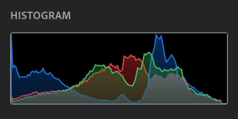
When working with data, visual exploration often helps you spot trends, patterns, or outliers faster than rows in a table. One of the most useful ways to visualize numerical data is through a histogram. In Python, Matplotlib.pyplot.hist() is the go-to function for plotting them. Whether you're analyzing exam scores, sensor readings, or anything else with continuous values, this method breaks down data into ranges (called bins). It shows how many data points fall into each. It’s simple, effective, and customizable. This article walks you through how plt.hist() works and how to control its appearance, step by step.

Getting Started with Matplotlib.pyplot.hist()

At its core, a histogram groups continuous data into bins and displays the frequency of values in each bin using bars. The Matplotlib.pyplot.hist() function does all this with minimal code. Here's a basic example:

python

CopyEdit

import matplotlib.pyplot as plt

import numpy as np

data = np.random.normal(loc=50, scale=10, size=1000)

plt.hist(data)

plt.show()

This script creates a Python histogram plot based on 1,000 random numbers drawn from a normal distribution. The default number of bins is 10, but you can control this with the bins parameter. For example, plt.hist(data, bins=20) splits the data into 20 segments. This affects the level of detail in the plot. If there are too few bins, you might miss important structures. Too many, and the plot can become noisy.

You can also input other arrays, such as integers or floats, directly from CSV files, DataFrames, or generated arrays. Matplotlib.pyplot.hist() accepts a list, NumPy array, or even Pandas Series. If the dataset is small, a histogram can reveal clustering, gaps, or uneven spread. If it’s large, the histogram gives a quick overview of the distribution's shape—whether it’s symmetric, skewed, bimodal, or uniform.

Customizing the Histogram for Better Insight

A histogram doesn’t have to be plain. You can tweak many visual elements using arguments within plt.hist(). These include color, transparency, orientation, and edge styling.

Let’s say you want to change the bar color, remove outlines, and make the bars semi-transparent:

python

CopyEdit

plt.hist(data, bins=15, color='skyblue', edgecolor='black', alpha=0.7)

plt.title("Test Score Distribution")

plt.xlabel("Score")

plt.ylabel("Frequency")

plt.grid(True)

plt.show()

In this example, alpha=0.7 controls transparency. This becomes useful when comparing multiple datasets in one plot. Use the label to give each set a name and plt.legend() to display them.

Orientation matters too. By default, histograms are vertical. You can make them horizontal using orientation='horizontal', which flips the axes. It might help if your value labels are long or your dataset is easier to interpret sideways.

One often overlooked setting is density=True. This normalizes the histogram so that the total area under the bars equals 1. It's useful when plotting probability density functions or when comparing datasets of different sizes. You’ll see relative proportions instead of raw counts.

For advanced users, cumulative=True turns the histogram into a cumulative distribution chart. This shows how the values accumulate over time or value ranges. It can be especially helpful in reliability studies or when tracking time-to-event data.

Binning Strategies and Frequency Counts

The choice of bin size influences how the Python histogram plot looks. A poor choice may misrepresent the data. If you don’t want to set bins manually, you can use predefined rules like 'auto', 'sturges', or 'fd', which automatically determine a suitable number based on the data.

python

CopyEdit

plt.hist(data, bins='sturges')

You can also manually provide bin edges using a list. For example, if your values range from 0 to 100 and you want to group them into decades, use:

python

CopyEdit

plt.hist(data, bins=[0,10,20,30,40,50,60,70,80,90,100])

Another trick involves pulling out the frequency data separately. Matplotlib.pyplot.hist() can return the counts, bin edges, and patches (visual elements). This gives you more control, especially when further processing is needed:

python

CopyEdit

counts, bin_edges, patches = plt.hist(data, bins=10)

You can use counts to label bars or apply conditional formatting—for instance, coloring bars differently if they exceed a threshold. This adds context and improves the plot’s ability to tell a story.

Histograms can also handle categorical data by assigning numeric values, but they're best suited for continuous ranges. For nominal data, bar plots are more appropriate.

Multiple Histograms and Overlay Techniques

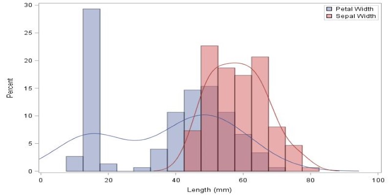
Sometimes it’s useful to compare multiple distributions. You can overlay histograms using transparency or stack them to show combined effects.

python

CopyEdit

data1 = np.random.normal(50, 10, 1000)

data2 = np.random.normal(60, 15, 1000)

plt.hist([data1, data2], bins=20, alpha=0.6, label=['Set A', 'Set B'])

plt.legend()

plt.show()

In this example, both sets share the same bins, which is important for comparison. Overlaying helps when the distributions have similar ranges, while stacked histograms are better for showing aggregate effects.

Python histogram plot comparisons can also benefit from cumulative and density overlays. You can add a line plot or a kernel density estimate (KDE) from libraries like seaborn or scipy to enhance readability, though Matplotlib.pyplot.hist() handles the base structure well.

Another useful tip is to limit the x or y axis using plt.xlim() and plt.ylim(). This is handy when outliers distort the view and you want to focus on the bulk of the data.

Finally, save your histograms using plt.savefig('histogram.png', dpi=300) for reports or sharing. Exporting at high resolution ensures your work remains clear in print or presentations.

Conclusion

Matplotlib.pyplot.hist() is a simple yet flexible tool for building histograms in Python. It’s quick to use and handles most of the formatting and binning automatically. With just a few optional parameters, it can go from basic to polished in just a few lines of code. Whether you need to spot patterns, compare datasets, explore distributions, or prepare figures for a report, this function gives you the structure and freedom to get it right. The key is to think about what you want to show, then use the right settings to make that visible. Histograms help your data speak clearly, one bin at a time.